By Ami Levin, SQL Server MVP
In the second part of this series on physical join operators we looked at the Merge Operator. In the final part of the series we turn our attention to the Hash operator.
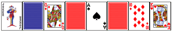
For this article series I am using an analogy of two sets of standard playing cards. One set with a blue back and another with a red back that need to be 'joined' together according to various join conditions. The two sets of cards simply represent the rows from the two joined tables, the red input and the blue input - "Now Neo - which input do you choose"?
The algorithm for a hash match join operator is a little more complicated:
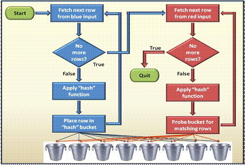
Each row in the blue input is fetched and a hash function (explained soon) is applied on the join expression. The row (in full, part or just a pointer) is placed in a 'bucket' which represents the result of the hash function. After all relevant rows have been 'hashed' and placed in their appropriate buckets; the rows from the red input are fetched one by one. For each row, the same hash function is applied to the join expression and matches are looked for (probed) within the appropriate bucket only. If we would use this operator to join our playing cards, we would need to decide on an appropriate hash function. For example, let's assume our hash function is the card's suit. In this case, we would first separate the blue-back cards into 4 piles (buckets) by suit - spades, clubs, hearts and diamonds. Then, we would pick the red-back cards, one by one, look at their suit and try to find their match within the appropriate pile only.
The tricky part of achieving high efficiency with the hash match operator is choosing the right hash function for a particular data set. This is a highly challenging task which is handled by expert mathematicians and is one of the most secret aspects of the query optimizer. Imagine what would happen, if in the card example above, we would use the same hash function (card suit) for a set of 1 million cards that consists of spades only... On the other hand, imagine what would happen if we used the same function when the same million cards consisted of a million different (hypothetical) suits? Remember that a join may be performed on any comparable data type with highly varying distribution patterns and with highly varying filter patterns... It's an extremely complicated and delicate balance.
The hash match operator has some additional overhead we need to consider as well. Besides the obvious CPU overhead for applying the potentially complicated hash function on every row in both inputs, memory pressures may have devastating performance results for this operator as well. The hash buckets must be persisted until the whole operation completes and all rows are matched. This requires significant memory resources, in addition to the actual data pages in the buffer cache. In case that memory is needed for other concurrent operations or in case there is simply not enough memory to hold all buckets for large hash joins, the buckets are flushed from cache and physically written to TempDB. Of course, they will need to be physically retrieved into memory when their content needs to be updated or probed which might prove to be quite painful for those people who like their results delivered in less time than if sent by first class mail. The query optimizer is aware of this fact and may consider the amount of free memory when deciding between hash match and alternative operators.
So when is a hash match join a good choice? Well, I would say far less than it's actually being used, and not due to the optimizer fault... The main advantage of hash match over nested loops is that the data is (seemingly) accessed only once. But, remember that the probing of the buckets is in fact repeated access of the data (or part of it) which does not constitute logical reads and therefore is a 'hidden' from our eyes and most monitoring tools. Hash match might be the best choice when both inputs are very large and using nested loops may cause 'a-sequential page flushes'. In most practical cases, the optimizer will revert to hash match when the inputs are not properly indexed (intentionally or not). Optimizing your indexes will, in many cases, cause the optimizer to change its choice of execution plans to use nested loops instead of hash match, significantly reducing CPU and memory consumption, potentially affecting the performance of the whole workload. Let's check out a few examples where the optimizer chooses to use hash match.
Hash Match used with very large inputs
The simplest case is when both inputs are simply too large for nested loops. In Query 8 , both inputs are ~120,000 rows (source not shown, but you can trust me). Although both are 'ideally' indexed for the join column and although the indexes cover the query so no lookups are required, nested loops will simply require too many iterations. Remember that even an efficient index seek might consist of a few page accesses for traversing the non leaf level of the index.
Query 8
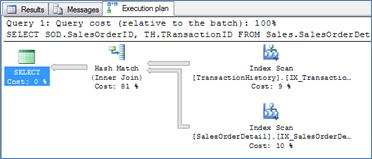
Execution Plan 8
Hash Match used when multiple lookups are the 2nd best alternative
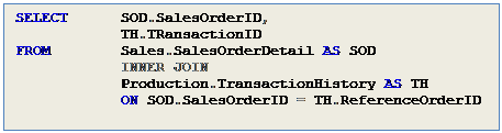
In Query 9 below, both inputs are not small enough (P ~500 rows, SOD ~120,000 rows) to make nested loops efficient. It's interesting to see that even though Product ID is indexed, nested loops will probably not be a good choice here. The main reason is that the index on Product ID does not cover the query andOrderQty will need to be looked up for each order which sums up to ~120,000 lookups.
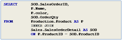
Query 9
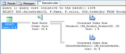
Execution Plan 9
* Exercise: In the demo code, you will find the same query without the OrderQty column in the select list (Query 9b). Try to guess what join operator will the optimizer choose when the need for lookups is eliminated? Try it…
Physical vs. Logical scan order
I would also like to draw your attention to another interesting property of the execution plan. If you look at the properties of either index scan above, you will see the value 'false' for the scan property 'ordered'.
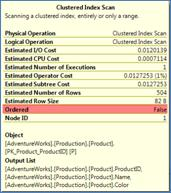
This means that the storage engine is not required to follow the logical chain links between the index leaf pages that point to the 'next' and 'previous' pages. Since the order of the retrieval of the rows is of no significance to the hash match operator, the storage engine will optimize the scan performance by scanning the index pages in their physical order (by following the IAM pages). This might prove to be a significant performance gain, especially for indexes with a high level of logical fragmentation. Go back and look at this property for index scans of the execution plans of the merge examples above.
Another thing we should note about hash joins is the fact that, in contrast to both nested loops and merge operators where the join operator may immediately start outputting joined rows for further processing, no rows can be outputted when using hash match until the whole 'blue input' is fully hashed.
Summary
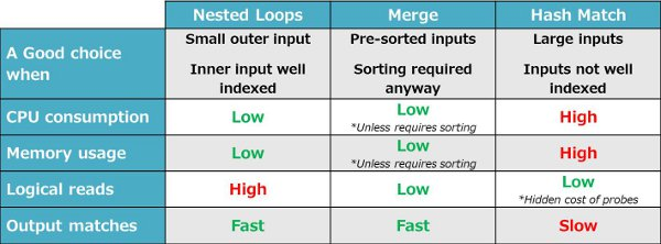
In a nutshell, we can sum up the main properties of the three physical operators available to the SQL Server optimizer when carrying out Equi-Inner-Joins.